501 時系列データ分析
読み込み
In [1]:
import os
import pandas as pd
import datetime as dt

import warnings
warnings.filterwarnings("ignore")

import matplotlib.pyplot as plt
import matplotlib.dates as mdates
%matplotlib inline

from matplotlib import pyplot
from statsmodels.graphics.tsaplots import plot_acf
from statsmodels.tsa.arima_model import ARIMA
時系列データの整形
時系列データの入手
Don’t spam this downloading
In [2]:
url = 'http://www.jepx.org/market/excel/spot_2017.csv'
spot_df = pd.read_csv(url, encoding='shift-jis', parse_dates=[0])
インデックスの整形
In [3]:
hm = spot_df.loc[:, '時刻コード']/2*60 - 30.0
h_list = []
for m in hm:
    h_list.append(dt.timedelta(minutes=m))

spot_df.index = pd.to_datetime(spot_df.loc[:, '年月日']) + h_list
del spot_df['年月日']
del spot_df['時刻コード']
spot_df.index.name = 'Datetime'

display(spot_df['2017-4-1 00:00:00':'2017-4-1 03:00:00'])
| 売り入札量(kWh) | 買い入札量(kWh) | 約定総量(kWh) | システムプライス(円/kWh) | エリアプライス北海道(円/kWh) | エリアプライス東北(円/kWh) | エリアプライス東京(円/kWh) | エリアプライス中部(円/kWh) | エリアプライス北陸(円/kWh) | エリアプライス関西(円/kWh) | ... | 回避可能原価全国値(円/kWh) | 回避可能原価北海道(円/kWh) | 回避可能原価東北(円/kWh) | 回避可能原価東京(円/kWh) | 回避可能原価中部(円/kWh) | 回避可能原価北陸(円/kWh) | 回避可能原価関西(円/kWh) | 回避可能原価中国(円/kWh) | 回避可能原価四国(円/kWh) | 回避可能原価九州(円/kWh) | |
|---|---|---|---|---|---|---|---|---|---|---|---|---|---|---|---|---|---|---|---|---|---|
| Datetime | |||||||||||||||||||||
| 2017-04-01 00:00:00 | 4812000 | 3765500 | 1319000 | 10.23 | 11.79 | 11.79 | 11.79 | 8.58 | 8.58 | 8.58 | ... | 10.26 | 11.80 | 11.79 | 11.79 | 8.55 | 8.58 | 8.65 | 8.58 | 8.58 | 7.12 |
| 2017-04-01 00:30:00 | 5082000 | 3663500 | 1243500 | 9.62 | 10.34 | 10.34 | 10.34 | 8.64 | 8.64 | 8.64 | ... | 9.63 | 10.34 | 10.29 | 10.31 | 8.70 | 8.74 | 8.69 | 8.64 | 8.64 | 6.27 |
| 2017-04-01 01:00:00 | 5717500 | 3594000 | 1186500 | 9.17 | 10.20 | 10.20 | 10.20 | 8.76 | 8.76 | 8.76 | ... | 9.21 | 10.20 | 10.20 | 10.16 | 8.78 | 8.93 | 8.81 | 8.76 | 8.76 | 7.13 |
| 2017-04-01 01:30:00 | 5926000 | 3634000 | 1154500 | 8.80 | 10.03 | 10.03 | 10.03 | 8.77 | 8.77 | 8.77 | ... | 8.87 | 10.03 | 10.04 | 10.00 | 8.80 | 8.95 | 8.82 | 8.77 | 8.77 | 7.13 |
| 2017-04-01 02:00:00 | 6164500 | 3682500 | 1158500 | 8.89 | 9.32 | 9.32 | 9.32 | 8.84 | 8.84 | 8.84 | ... | 8.92 | 9.33 | 9.36 | 9.33 | 8.87 | 8.87 | 8.90 | 8.84 | 8.84 | 7.12 |
| 2017-04-01 02:30:00 | 6177000 | 3674500 | 1355000 | 8.69 | 9.01 | 8.69 | 8.69 | 8.69 | 8.69 | 8.69 | ... | 8.72 | 9.01 | 8.70 | 8.73 | 8.72 | 8.75 | 8.75 | 8.69 | 8.69 | 7.12 |
| 2017-04-01 03:00:00 | 6334500 | 3658500 | 1414000 | 8.64 | 9.01 | 8.65 | 8.65 | 8.65 | 8.65 | 8.65 | ... | 8.67 | 9.01 | 8.66 | 8.70 | 8.69 | 8.71 | 8.72 | 8.65 | 8.65 | 7.12 |
7 rows × 30 columns
必要なカラムの抽出
In [4]:
target_column = 'エリアプライス東京(円/kWh)'
target_df = pd.DataFrame(spot_df.loc['2017-04-01':'2017-12-31', target_column].copy())
target_df.indexes = ['Datetime']
target_df.columns = ['E_RATE']

display(target_df['2017-4-1 00:00:00':'2017-4-1 03:00:00'])
| E_RATE | |
|---|---|
| Datetime | |
| 2017-04-01 00:00:00 | 11.79 |
| 2017-04-01 00:30:00 | 10.34 |
| 2017-04-01 01:00:00 | 10.20 |
| 2017-04-01 01:30:00 | 10.03 |
| 2017-04-01 02:00:00 | 9.32 |
| 2017-04-01 02:30:00 | 8.69 |
| 2017-04-01 03:00:00 | 8.65 |
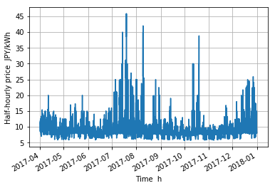
グラフ化
年間
In [5]:
fig = plt.figure()
ax = fig.add_subplot(111)

x_text = 'Time  h'
y_text = 'Half-hourly price  JPY/kWh'
plt.xlabel(x_text)
plt.ylabel(y_text)

ax.xaxis.set_minor_locator(mdates.MonthLocator())
ax.format_xdata = mdates.DateFormatter('%m')
fig.autofmt_xdate()

plt.plot(target_df)
plt.grid()
plt.show()
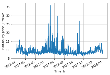
移動平均
Rolling average
In [6]:
fig = plt.figure()
ax = fig.add_subplot(111)

x_text = 'Time  h'
y_text = 'Half-hourly price  JPY/kWh'
plt.xlabel(x_text)
plt.ylabel(y_text)

ax.xaxis.set_minor_locator(mdates.MonthLocator())
ax.format_xdata = mdates.DateFormatter('%m')
fig.autofmt_xdate()

plt.plot(target_df['E_RATE'].rolling(window=24, min_periods=2).mean())
plt.grid()
plt.show()
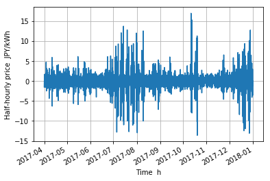
差分
first order difference
In [7]:
fig = plt.figure()
ax = fig.add_subplot(111)

x_text = 'Time  h'
y_text = 'Half-hourly price  JPY/kWh'
plt.xlabel(x_text)
plt.ylabel(y_text)

ax.xaxis.set_minor_locator(mdates.MonthLocator())
ax.format_xdata = mdates.DateFormatter('%m')
fig.autofmt_xdate()

plt.plot(target_df['E_RATE'].diff())
plt.grid()
plt.show()
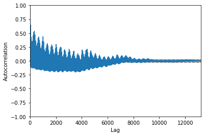
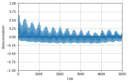
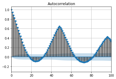
自己相関
Autocorrelation
In [8]:
display(target_df['E_RATE'].autocorr())

pd.plotting.autocorrelation_plot(target_df['E_RATE'])
plt.grid()
plt.show()

pd.plotting.autocorrelation_plot(target_df['E_RATE'])
plt.xlim(0,5000)
plt.show()
0.9430484073963505
In [9]:
plot_acf(target_df['E_RATE'])
plt.xlim(0,100)
plt.grid()
plt.show()
自己回帰和分移動平均モデル
Autoregressive Integrated Moving Average (ARIMA)
In [10]:
ar = 5 # Autoregressive model(AR)
i = 1  # Integrated model (I)
ma = 1 # Moving Average (MA)

model_arima = ARIMA(target_df['E_RATE'], order=(ar, i, ma))
model_fit = model_arima.fit(disp=0)
display(model_fit.summary())
| Dep. Variable: | D.E_RATE | No. Observations: | 13199 |
|---|---|---|---|
| Model: | ARIMA(5, 1, 1) | Log Likelihood | -20646.580 |
| Method: | css-mle | S.D. of innovations | 1.156 |
| Date: | Fri, 11 May 2018 | AIC | 41309.160 |
| Time: | 13:24:20 | BIC | 41369.063 |
| Sample: | 04-01-2017 | HQIC | 41329.160 |
| - 12-31-2017 |
| coef | std err | z | P>|z| | [0.025 | 0.975] | |
|---|---|---|---|---|---|---|
| const | -2.919e-05 | 0.000 | -0.075 | 0.940 | -0.001 | 0.001 |
| ar.L1.D.E_RATE | 0.9830 | 0.009 | 112.771 | 0.000 | 0.966 | 1.000 |
| ar.L2.D.E_RATE | -0.0249 | 0.012 | -2.043 | 0.041 | -0.049 | -0.001 |
| ar.L3.D.E_RATE | 0.0448 | 0.012 | 3.675 | 0.000 | 0.021 | 0.069 |
| ar.L4.D.E_RATE | -0.0287 | 0.012 | -2.354 | 0.019 | -0.053 | -0.005 |
| ar.L5.D.E_RATE | -0.0543 | 0.009 | -6.232 | 0.000 | -0.071 | -0.037 |
| ma.L1.D.E_RATE | -0.9970 | 0.001 | -1400.813 | 0.000 | -0.998 | -0.996 |
| Real | Imaginary | Modulus | Frequency | |
|---|---|---|---|---|
| AR.1 | 1.1367 -0.0000j 1.1367 -0.0000||||
| AR.2 | 1.5202 -0.0000j 1.5202 -0.0000||||
| AR.3 | -0.3333 -2.0298j 2.0570 -0.2759||||
| AR.4 | -0.3333 +2.0298j 2.0570 0.2759||||
| AR.5 | -2.5188 -0.0000j 2.5188 -0.5000||||
| MA.1 | 1.0030 +0.0000j 1.0030 0.0000
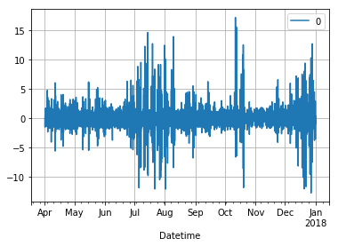
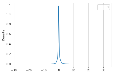
残差
In [11]:
residuals = pd.DataFrame(model_fit.resid)
residuals.plot()
plt.grid()
plt.show()

residuals.plot(kind='kde')
plt.grid()
plt.show()
display(residuals.describe())
| 0 | |
|---|---|
| count | 13199.000000 |
| mean | -0.000082 |
| std | 1.156389 |
| min | -12.765292 |
| 25% | -0.224910 |
| 50% | -0.058646 |
| 75% | 0.140634 |
| max | 17.109040 |