602 Satisfiable Modulo Theories(SMT)

PREPARATION

pip install z3-solver

Example: Tonkoke

http://mechlog.jp/materials/601_Linear_programming.html

\[ \begin{align}\begin{aligned}\exists x_1 \exists x_2 \exists x_3 \varphi(y,x_1,x_2, x_3)\\where\end{aligned}\end{align} \]

\[\begin{split}\varphi(y,x_1,x_2, x_3) = (y=15x_1+18x_2+30x_3 \wedge \\ 2x_1+x_2+x_3 \le 60 \wedge \\ x_1+2x_2+x_3 \le 60 \wedge \\ x_3 \le 30 \wedge \\ x_1, x_2, x_3 \ge 0)\end{split}\]

To parametric Optimization problem

\[\begin{split}\varphi(y,x_1,x_2, x_3) = (y=15x_1+18x_2+30x_3 \wedge \\ 2x_1+x_2+x_3 \le 60 \wedge \\ x_1+2x_2+x_3 \le 60 + {\color{red}{\theta_1}} \wedge \\ x_3 \le 30 \wedge \\ x_1, x_2, x_3 \ge 0)\end{split}\]

Developler of SAT/SMT solver named Z3:

https://stackoverflow.com/users/1096362/nikolaj-bjorner

Description example of Z3:

e.g. ForAll([x], Implies(x >= 25, Exists([u,v], And(u >= 0, v >= 0, x == 3u + 5v))))

Import

import z3
import numpy as np
import matplotlib.pyplot as plt
%matplotlib inline
import warnings
warnings.filterwarnings("ignore")

Define functions

def make_vars():
    x1, x2, x3, y, theta1 = z3.Reals('x1 x2 x3 y theta1')
    return x1, x2, x3, y, theta1

def check_feasibility(funcs):
    solver = z3.Solver()
    solver.add(funcs)
    return solver.check(), solver.model()

def maximize(problem, obj_func):
    model = z3.Optimize()
    model.add(problem)
    model.maximize(obj_func)
    return model.check(), model.model()

def eliminate(problem):
    return z3.simplify(z3.Tactic('qe')(problem).as_expr())

Problem definition

def make_problem_with_sensitivity_parameters(x1, x2, x3, y, theta1):
    return z3.Exists([x1, x2, x3], z3.And(15*x1 + 18*x2 + 30*x3 == y,
                                           2*x1 + x2 + x3 <= 60,
                                           x1 + 2*x2 + x3 <= 60 + theta1,
                                                       x3 <= 30,
                                           x1 >=0, x2 >=0, x3 >=0
                                          )
                     )

def make_problem(x1, x2, x3, y):
    return z3.Exists([x1, x2, x3], z3.And(15*x1 + 18*x2 + 30*x3 == y,
                                           2*x1 + x2 + x3 <= 60,
                                           x1 + 2*x2 + x3 <= 60,
                                                       x3 <= 30,
                                           x1 >=0, x2 >=0, x3 >=0
                                          )
                     )

Execution

x1, x2, x3, y, theta1 = make_vars()
original_problem = make_problem(x1, x2, x3, y)
sensitivity_analysis = make_problem_with_sensitivity_parameters(x1, x2, x3, y, theta1)

print('=== Evaluate whether feasible problem ===')
print(check_feasibility(original_problem))
print(check_feasibility(sensitivity_analysis))

print('=== Optimize the problem ===')
print(maximize(original_problem, y))

print('=== Do QE to the problem ===')
print(eliminate(sensitivity_analysis))

=== Evaluate whether feasible problem ===
(sat, [y = 0])
(sat, [y = 0, theta1 = -60])
=== Optimize the problem ===
(sat, [y = 1230])
=== Do QE to the problem ===
Or(And(Not(y >= 1440),
       Not(650/7 <= 5/63*y + -5/7*theta1),
       y >= 900),
   And(y <= 1800,
       1/42*y + -5/7*theta1 <= 300/7,
       Not(y >= 900),
       y >= 0),
   And(Not(y >= 1800),
       Not(300/7 <= 1/42*y + -5/7*theta1),
       y <= 900,
       Not(y <= 0)),
   And(Not(y >= 1440),
       5/36*y + -5/4*theta1 <= 325/2,
       Not(y <= 900)),
   And(Not(3075/14 <= 5/28*y + -5/4*theta1),
       Not(-325/2 <= -5/36*y + 5/4*theta1),
       Not(225/2 <= 1/12*y + -5/4*theta1)),
   And(5/28*y + -5/4*theta1 <= 3075/14,
       Not(-325/2 <= -5/36*y + 5/4*theta1),
       1/12*y + -5/4*theta1 <= 225/2),
   And(y <= 1440, 5/36*y + -5/4*theta1 <= 325/2, y >= 900),
   And(Not(-750/7 <= -5/84*y + -5/7*theta1),
       Not(y >= 1440),
       Not(y >= 1800),
       y >= 1080),
   And(Not(y >= 1080),
       Not(300/7 <= 5/63*y + -5/7*theta1),
       Not(y <= 0)),
   And(5/84*y + 5/7*theta1 <= 750/7,
       Not(650/7 <= 5/63*y + -5/7*theta1),
       Not(300/7 <= 1/42*y + -5/7*theta1),
       -5/63*y + 5/7*theta1 <= -300/7),
   And(Not(3075/14 <= 5/28*y + -5/4*theta1),
       -5/36*y + 5/4*theta1 <= -325/2,
       Not(225/2 <= 1/12*y + -5/4*theta1)),
   And(Not(y >= 1440),
       Not(325/2 <= 5/36*y + -5/4*theta1),
       y >= 900))

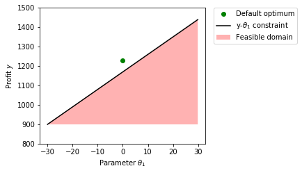
Visualize

fig, ax = plt.subplots()
ax.plot(0, 1230, 'o', color='green', label='Default optimum')

y_fill = np.arange(900, 1440, 1)#900 <= y <= 1440
x_fill = (5/36*y_fill - 325/2)*(4/5)# theta1 >= (5/36*y - 325/2)*4/5
ax.plot(x_fill, y_fill, color='black', label=r'y-$\theta_1$ constraint')
plt.fill_between(x_fill, y_fill, 900, where=y_fill<=1440, facecolor='red',
                 alpha=0.3, label='Feasible domain')
ax.set_ylim(800,1500)
ax.set_xlabel(r'Parameter $ \theta_1 $')
ax.set_ylabel(r'Profit $ y $')

plt.subplots_adjust(left = 0.20, right = 0.75, bottom=0.2)
plt.legend(bbox_to_anchor=(1.05, 1), loc='upper left',
           borderaxespad=0, fontsize=10)
plt.plot()

[]