221 ランキンサイクル
Example: Non-ideal Rankine cycle
読み込み
In [3]:
import numpy as np
import pandas as pd

import CoolProp.CoolProp as CP

import matplotlib.pyplot as plt
%matplotlib inline
import warnings
warnings.filterwarnings("ignore")
パラメータ定義
In [4]:
WF = 'water'

T_H = 800 # K
T_C = 325 # K
P_b = 2.64 *10**6 # Pa
ETA_turbine = 0.85
ETA_pump = 0.65
DT_cond = 7 # K
DT_b = 35# K
DP_cond = 4.5 *10**3 # Pa
DP_b = 792 *10**3 # Pa
データフレーム用意
In [5]:
index = list(range(1,4+1))
states = pd.DataFrame(columns=['T', 'P', 's', 'v', 'h', 'x', 's_s', 'h_s'], index=index)#K, Pa, J/kg/K, m3, J/kg, [-], [], []
Point 2: Boiler exit/Turbine inlet
In [6]:
states.loc[2, 'P'] = P_b - DP_b
states.loc[2, 'T'] = T_H - DT_b
states.loc[2, 'h'] = CP.PropsSI('H', 'P', states.loc[2, 'P'], 'T', states.loc[2, 'T'], WF)
states.loc[2, 's'] = CP.PropsSI('S', 'P', states.loc[2, 'P'], 'T', states.loc[2, 'T'], WF)
Point 4: Condenser exit/Pump inlet
In [7]:
states.loc[4, 'x'] = 0
states.loc[4, 'T'] = T_C + DT_cond
states.loc[4, 's'] = CP.PropsSI('S', 'Q', states.loc[4, 'x'], 'T', states.loc[4, 'T'], WF)
states.loc[4, 'h'] = CP.PropsSI('H', 'Q', states.loc[4, 'x'], 'T', states.loc[4, 'T'], WF)
states.loc[4, 'P'] = CP.PropsSI('P', 'Q', states.loc[4, 'x'], 'T', states.loc[4, 'T'], WF)
states.loc[4, 'v'] = CP.PropsSI('V', 'Q', states.loc[4, 'x'], 'T', states.loc[4, 'T'], WF)
Point 1: Pump exit/Boiler inlet
In [8]:
states.loc[1, 'P'] = P_b
states.loc[1, 's_s'] = states.loc[4, 's']
states.loc[1, 'h_s'] = CP.PropsSI('H', 'S', states.loc[1, 's_s'], 'P', states.loc[1, 'P'], WF)
W_dot_s_p_m_dot = states.loc[1, 'h_s'] - states.loc[4, 'h']
W_dot_p_m_dot = W_dot_s_p_m_dot / ETA_pump
states.loc[1, 'h'] = states.loc[4, 'h'] + W_dot_p_m_dot
states.loc[1, 's'] = CP.PropsSI('S', 'H', states.loc[1, 'h'], 'P', states.loc[1, 'P'], WF)
states.loc[1, 'T'] = CP.PropsSI('T', 'H', states.loc[1, 'h'], 'P', states.loc[1, 'P'], WF)
Point 3: Turbine exit/Condenser inlet
In [9]:
states.loc[3, 'P'] = states.loc[4, 'P'] + DP_cond
states.loc[3, 's_s'] = states.loc[2, 's']
states.loc[3, 'h_s'] = CP.PropsSI('H', 'S', states.loc[3, 's_s'], 'P', states.loc[3, 'P'], WF)
W_dot_s_t_m_dot = states.loc[2, 'h'] - states.loc[3, 'h_s']
W_dot_t_m_dot = W_dot_s_t_m_dot * ETA_turbine
states.loc[3, 'h'] = states.loc[2, 'h'] - W_dot_t_m_dot
states.loc[3, 's'] = CP.PropsSI('S', 'H', states.loc[3, 'h'], 'P', states.loc[3, 'P'], WF)
states.loc[3, 'T'] = CP.PropsSI('T', 'H', states.loc[3, 'h'], 'P', states.loc[3, 'P'], WF)
states.loc[3, 'x'] = CP.PropsSI('Q', 'H', states.loc[3, 'h'], 'P', states.loc[3, 'P'], WF)
In [10]:
display(states)
| T | P | s | v | h | x | s_s | h_s | |
|---|---|---|---|---|---|---|---|---|
| 1 | 332.452 | 2.64e+06 | 821.138 | NaN | 250464 | NaN | 816.823 | 249030 |
| 2 | 765 | 1.848e+06 | 7448.51 | NaN | 3.45198e+06 | NaN | NaN | NaN |
| 3 | 341.67 | 23408.6 | 7881.91 | NaN | 2.62477e+06 | -1 | 7448.51 | 2.47879e+06 |
| 4 | 332 | 18908.6 | 816.823 | 0.000474239 | 246367 | 0 | NaN | NaN |
Component energy balances
In [11]:
Q_dot_b_m_dot = states.loc[2, 'h'] - states.loc[1, 'h']
Q_dot_cond_m_dot = states.loc[3, 'h'] - states.loc[4, 'h']
check_1 = W_dot_t_m_dot + Q_dot_cond_m_dot \
            - W_dot_p_m_dot - Q_dot_b_m_dot
print(Q_dot_b_m_dot, Q_dot_cond_m_dot, check_1)
3201517.4577735155 2378404.3311674045 0.0
In [12]:
W_dot_net_m_dot = W_dot_t_m_dot - W_dot_p_m_dot
ETA_Rankine = W_dot_net_m_dot / Q_dot_b_m_dot
bwr = W_dot_p_m_dot / W_dot_t_m_dot
heat_rate_BtuoKWhr = Q_dot_b_m_dot / W_dot_net_m_dot
print(W_dot_net_m_dot, ETA_Rankine, bwr, heat_rate_BtuoKWhr)
823113.1266061105 0.25710093337380757 0.004952554476169804 3.889523024586094
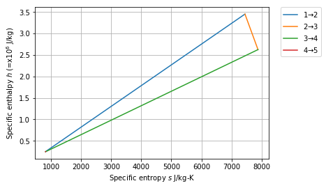
h-s chart
In [13]:
nb_points = 1000
h12 = np.linspace(states.ix[1, 'h'], states.ix[2, 'h'], nb_points)
h23 = np.linspace(states.ix[2, 'h'], states.ix[3, 'h'], nb_points)
h34 = np.linspace(states.ix[3, 'h'], states.ix[4, 'h'], nb_points)
h41 = np.linspace(states.ix[4, 'h'], states.ix[1, 'h'], nb_points)

s12 = np.linspace(states.ix[1, 's'], states.ix[2, 's'], nb_points)
s23 = np.linspace(states.ix[2, 's'], states.ix[3, 's'], nb_points)
s34 = np.linspace(states.ix[3, 's'], states.ix[4, 's'], nb_points)
s41 = np.linspace(states.ix[4, 's'], states.ix[1, 's'], nb_points)
L_h = [h12, h23, h34, h41]
L_s = [s12, s23, s34, s41]

for i in range(len(L_s)):
    plt.plot(L_s[i],L_h[i]/1e6,label='{}$\\to${}'.format(i+1,(i+1)%5+1))

plt.legend(bbox_to_anchor=(1.05, 1), loc='upper left', borderaxespad=0)
plt.xlabel('Specific entropy $s$ J/kg-K')
plt.ylabel('Specific enthalpy $h$ (=x$10^6$ J/kg)')
plt.grid()
plt.show()